Joining tables

Overview

Teaching: 20 min
Exercises: 15 min

Questions

• How to join different tables together?

• How to identify mis-matches between tables?

Objectives

• Apply the *_join() family of functions to merge two tables with each other.

• Use anti_join() to identify non-matches between two tables.

• Recognise when to use each kind of joinining operation.

In this lesson we’re going to learn how to use functions from the dplyr package (part of tidyverse) to help us combine different tables together.

As usual when starting an analysis on a new script, let’s start by loading the packages and reading the data. In this case, let’s use the clean dataset that we created in the last exercise of our previous episode.

# load the package
library(tidyverse)
# Read the data, specifying how missing values are encoded
gapminder_clean <- read_csv("data/processed/gapminder1960to2010_socioeconomic_clean.csv", 
                            na = "")

If you haven’t completed that exercise, here’s how you can recreate the clean dataset:

gapminder_clean <- read_csv("data/raw/gapminder1960to2010_socioeconomic.csv", na = "") %>% 
 # fix typos in main_religion and world region
 mutate(main_religion = str_to_title(str_squish(main_religion)),
        world_region = str_to_title(str_replace_all(world_region, "_", " "))) %>% 
 # fit typos in income groups, which needs more steps
 mutate(income_groups = str_remove(income_groups, "_income")) %>% 
 mutate(income_groups = str_to_title(str_replace_all(income_groups, "_", " "))) %>% 
 # fix/create numeric variables
 mutate(life_expectancy_female = as.numeric(life_expectancy_female),
        life_expectancy_male = ifelse(life_expectancy_male == -999, NA, life_expectancy_male))

Joining tables

A common task in data analysis is to bring different datasets together, so that we can combine columns from two (or more) tables together.

This can be achieved using the join family of functions in dplyr. There are different types of joins, which can be represented by a series of Venn diagrams:

In the apendix exercises we’ve been exploring a dataset related to energy consumption in different counties. Let’s see how we can join these two datasets together, so that we have all information in a single table.

First, let’s start by reading the data into R (if you don’t have these data right-click this link, choose “Save link as…” and save it on the data/raw folder of your project directory):

# it's a tab-separated file, so we use read_tsv
energy <- read_tsv("data/raw/gapminder1990to2010_energy.tsv", 
                   na = "")

A critical step when joining tables is to identify which columns are used to “match” the rows between them (in databases these are referred to as key variables). In our case the columns country, world_region and year should, together, have a one-to-one match between our two tables.

We can quickly check that not all countries from gapminder_clean are present in the energy table (here we use the base R method of accessing columns with $, which returns a vector):

# the `all()` function checks whether all values of a logical vector are TRUE
all(gapminder_clean$country %in% energy$country)

[1] FALSE

And the same happens for year:

all(gapminder_clean$year %in% energy$year)

[1] FALSE

So, different types of join operations (represented in the figure above) will result in different outcomes.

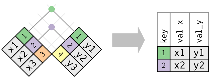
Let’s start by doing an inner join, which retains only the entries common to both tables:

inner_join(gapminder_clean, energy, 
           by = c("country", "world_region", "year"))

# A tibble: 3,990 x 16
   country world_region  year children_per_wo… life_expectancy income_per_pers…
   <chr>   <chr>        <dbl>            <dbl>           <dbl>            <dbl>
 1 Afghan… South Asia    1990             7.47            52.6             1861
 2 Afghan… South Asia    1991             7.48            52.4             1645
 3 Afghan… South Asia    1992             7.5             52.9             1522
 4 Afghan… South Asia    1993             7.54            53.2             1009
 5 Afghan… South Asia    1994             7.57            52.7              721
 6 Afghan… South Asia    1995             7.61            53.3             1028
 7 Afghan… South Asia    1996             7.63            53.8              942
 8 Afghan… South Asia    1997             7.64            53.7              865
 9 Afghan… South Asia    1998             7.62            52.8              800
10 Afghan… South Asia    1999             7.57            54.4              735
# … with 3,980 more rows, and 10 more variables: is_oecd <lgl>,
#   income_groups <chr>, population <dbl>, main_religion <chr>,
#   child_mortality <dbl>, life_expectancy_female <dbl>,
#   life_expectancy_male <dbl>, yearly_co2_emissions <dbl>,
#   energy_use_per_person <dbl>, energy_production_per_person <chr>

The by option is used to tell the join function which column(s) are used to “match” the rows of the two tables. We can see that the output has fewer rows than both of these tables, which makes sense given we’re only keeping the “intersection” between the two. Schematically, this is what happened:

The other types of join functions work exactly the same as this one, the only thing that changes is what kind of output you get. Schematically:

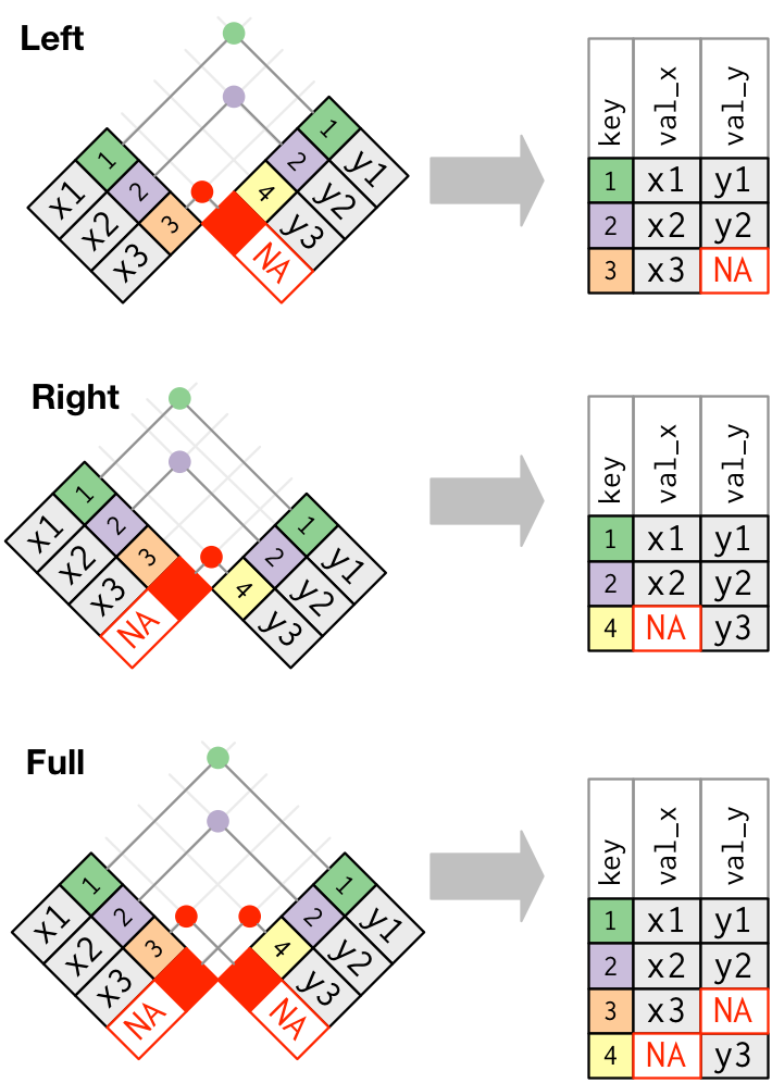
One important thing to note is that when doing either of these types of joins, the functions will take care of filling in the table with missing values, NA, whenever a row in one table does not have a match in the other table.

Exercise

1. Create a new table called gapminder_all, which includes all rows from both tables joined together by their common variable keys. Make a note of how many rows you have in the new table, and compare it with the original tables.
2. Use the anti_join() function to identify which rows in the energy dataset do NOT have a match in our original data.

Answer

A1.

Consulting the Venn diagrams at the top of the lesson, to retain all data from both tables, we should use the full_join() function (corresponding to an union of the two tables):

gapminder_all <- full_join(gapminder_clean, energy, by = c("country", "year", "world_region"))

# check how many rows
nrow(gapminder_all)

[1] 9844

This table has more rows than either of the original tables. This must be because some data exists in one table but not the other.

A2.

Again, the Venn diagram at the top of the page illustrates the result of an anti_join(), which we can apply to investigate this issue:

anti_join(energy, gapminder_clean, by = c("country", "year", "world_region"))

# A tibble: 1 x 6
  country world_region  year yearly_co2_emiss… energy_use_per_… energy_producti…
  <chr>   <chr>        <dbl>             <dbl>            <dbl> <chr>           
1 Brasil  America       1995           255793.             994. 0.00069         

We could further pipe (%>%) the output of the above operation to distinct() to check which countries were present in energy but missing in gapminder_clean:

# take the energy data frame, and then...
energy %>% 
  # anti join it with gapminder_clean, and then...
  anti_join(gapminder_clean, by = c("country", "world_region", "year")) %>% 
  # get the distinct values of country
  distinct(country)

# A tibble: 1 x 1
  country
  <chr>  
1 Brasil 

Note that if we dug a bit deeper into this, we would find that the country “Brasil” does occur in gapminder_clean, but it’s recorded as “Brazil”, so it’s a spelling inconsistency between the two datasets (in fact, the energy table has both “Brasil” and “Brazil”, which we should correct if we were analysing these data further).

Data tip: linking datasets

Combining datasets together is a very common task in data analysis, often referred to as data linkage.

Although this task might seem easy at a first glance, it can be quite challenging due to unforeseen properties of the data. For example:

• which variables in one table have a correspondence in the other table? (having the same column name doesn’t necessarily mean they are the same)
• are the values encoded similarly across datasets? (for example, one dataset might encode income groups as “low”, “medium”, “high” and another as “1”, “2”, “3”)
• were the data recorded in a consistent manner? (for example, an individual’s age might have been recorded as their date of birth or, due to confidentiality reasons, their age the last time they visited a clinic)

Thinking of these (and other) issues can be useful in order to avoid them when collecting your own data. Also, when you share data, make sure to provide with metadata, explaining as much as possible what each of your variables is and how it was measured.

Finally, it’s worth thinking that every observation of your data should have a unique identifier (this is referred to as a “primary key”). For example, in our data, a unique identifier could be created by the combination of the country and year variables, as those two define our unit of study in this case.

Key Points

• Use full_join(), left_join(), right_join() and inner_join() to merge two tables together.

• Specify the column(s) to match between tables using the by option.

• Use anti_join() to identify the rows from the first table which do not have a match in the second table.