Basic objects and data types in R

Overview

Teaching: 20 min
Exercises: 10 min

Questions

• What are the basic data structures and data types in R?

• How can values be assigned to objects?

• How can subsets be extracted from vectors?

• How are missing values represented in R?

Objectives

• Assign values to objects in R.

• Use functions and access their documentation.

• Distinguish between the following terms: object, assign, function, arguments, options.

• Understand and distinguish between two fundamental vector types: numeric and character.

• Subset and extract values from vectors.

• Understand how missing values are encoded in R.

Creating Objects in R

Often, you want to save the output of an operation for later use. In other words, we need to assign values to objects. To create an object, we need to give it a name followed by the assignment operator <-, and the value we want to give to it.

For example:

area_hectares <- 1

We can read the code as: the value 1 is assigned to the object area_hectares. Note that when you run this line of code the object you just created appears on your environment tab (top-right panel).

When assigning a value to an object, R does not print anything on the console. You can print the value by typing the object name on the console:

area_hectares

[1] 1

How should I name objects?

Object names can contain letters, numbers, underscores and periods. They cannot start with a number nor contain spaces. Different people use different conventions for long variable names, two common ones being:

• Underscore: my_long_named_object
• Camel case: myLongNamedObject

What you use is up to you, but be consistent. Also note that R is case-sensitive so area_hectares is different from Area_hectares.

Now that R has area_hectares in memory, we can do operations with it. For instance, we may want to convert this area into acres (area in acres is 2.47 times the area in hectares):

2.47 * area_hectares

[1] 2.47

We can also change an object’s value by assigning it a new one:

area_hectares <- 2.5
2.47 * area_hectares

[1] 6.175

Finally, assigning a value to one object does not change the values of other objects. For example, let’s store the plot’s area in acres in a new object, area_acres:

area_acres <- 2.47 * area_hectares

and then change area_hectares to 50.

area_hectares <- 50

Note that this did not change the value of area_acres.

Keyboard shortcut

In RStudio, the keyboard shortcut for <- is Alt + -.

Exercise

What is the value of bmi after running the following four lines of code:

weight_kg <- 70
height_m <- 1.80
bmi <- weight_kg/(height_m^2)
weight_kg <- 62

Solution

The value of bmi is 21.6 because it’s the result of 70/(1.8^2). Changing the weight_kg afterwards did not affect the bmi object.

Functions and Their Arguments

Functions perform specific operations or tasks in R. A function usually gets one or more inputs called arguments and returns a value. A typical example would be the function sqrt(). The input (the argument) must be a number, and the return value (the output) is the square root of that number. Executing a function (‘running it’) is refered to as calling the function. An example of a function call is:

b <- sqrt(a)

Here, the value of a is given to the sqrt() function, the sqrt() function calculates the square root, and returns the value which is then assigned to the object b. This function is very simple, because it takes just one argument.

The return value of a function need not be numerical (like that of sqrt()), and it also does not need to be a single item: it can be a set of things, or even a dataset. We’ll see that when we read data files into R.

Arguments can be anything, not only numbers or filenames, but also other objects. Exactly what each argument means differs per function, and must be looked up in the documentation (detailed below). Some functions take arguments which may either be specified by the user, or, if left out, take on a default value: these are called options. Options are typically used to alter the way the function operates.

Let’s try a function that can take multiple arguments:

round(3.14159)  # round a number

[1] 3

Here, we’ve called round() with just one argument, 3.14159, and it has returned the value 3. That’s because the default is to round to the nearest whole number. If we want more digits we can see how to do that by getting information about the round function. We can look at the help of any function by typing ? followed by the function’s name. In this case:

?round

We see that if we want a different number of digits, we can type digits = 2 or however many we want.

round(3.14159, digits = 2)

[1] 3.14

If you provide the arguments in the exact same order as they are defined you don’t have to name them:

round(3.14159, 2)

[1] 3.14

And if you do name the arguments, you can switch their order:

round(digits = 2, x = 3.14159)

[1] 3.14

It’s good practice to put the non-optional arguments (like the number you’re rounding) first in your function call, and to specify the names of all optional arguments. If you don’t, someone reading your code might have to look up the definition of a function with unfamiliar arguments to understand what you’re doing.

Vectors and Data Types

A vector is the most common and basic data structure in R. It consists of a collection of values that can be created with the c() function. For example:

some_numbers <- c(62, 77, 0, 6)
some_numbers

[1] 62 77  0  6

A vector can also contain character values, for example:

some_animals <- c("cat", "dog", "giraffe", "dog")
some_animals

[1] "cat"     "dog"     "giraffe" "dog"    

The quotes "" are essential here. Without the quotes R will assume there are objects called cat, dog and giraffe. As these objects don’t exist in R’s memory, there would be an error message.

There are many functions that allow you to inspect the content of a vector. length() tells you how many elements are in a particular vector:

length(some_numbers)

[1] 4

The function class() indicates what kind of object it is:

class(some_numbers)

[1] "numeric"

class(some_animals)

[1] "character"

Data types in R

The main data types in R are:

• numeric or double (a number with decimal points)
• integer (a number with no decimal points)
• character
• logical: TRUE or FALSE (we will discuss these in a future episode)

You can use the c() function to add other elements to your vector:

c(some_animals, "ant", "fruit fly")

[1] "cat"       "dog"       "giraffe"   "dog"       "ant"       "fruit fly"

Or even combine vectors together:

c(some_animals, some_animals)

[1] "cat"     "dog"     "giraffe" "dog"     "cat"     "dog"     "giraffe"
[8] "dog"    

Creating sequences of numbers

There are several shortcuts to create sequences of numbers, and these can be very useful in different situations:

1:10                           # integers from 1 to 10
10:1                           # integers from 10 to 1
seq(1, 10, by = 2)             # from 1 to 10 by steps of 2
seq(10, 1, by = -0.5)          # from 10 to 1 by steps of -0.5
seq(1, 10, length.out = 20)    # 20 equally spaced values from 1 to 10

Subsetting Vectors

If we want to extract one or several values from a vector, we must provide one or several indices in square brackets []. For instance:

some_animals <- c("cat", "dog", "giraffe", "dog")

# the second element of the vector
some_animals[2]

[1] "dog"

# the third and second elements of the vector
some_animals[c(3, 2)]

[1] "giraffe" "dog"    

We can also repeat the indices to create an object with more elements than the original one:

some_animals[c(1, 2, 2, 3, 3)]

[1] "cat"     "dog"     "dog"     "giraffe" "giraffe"

Vectorised operations

R deals with vector operations in a special way. Let’s take the addition of two numeric vectors as an example.

When operating on two vectors of the same length, R takes the elements of each vector one by one:

c(10, 20, 30, 40) + c(1, 2, 3, 4)  # equivalent to c(10 + 1, 20 + 2, 30 + 3, 40 + 4)

[1] 11 22 33 44

When operating on two vectors of different lengths, R will “recycle” the shortest vector (that is, it goes back to the start of the shortest vector when it runs out of values to pair with the longest vector):

c(10, 20, 30, 40) + c(1, 2)  # equivalent to c(10 + 1, 20 + 2, 30 + 1, 40 + 2)

[1] 11 22 31 42

This means that if we add a single number to a numeric vector, then R adds it to every value of the vector (because it “recycles” that single value every time):

c(10, 20, 30, 40) + 1  # equivalent to c(10 + 1, 20 + 1, 30 + 1, 40 + 1)

[1] 11 21 31 41

Missing Data

As R was designed to analyze datasets, it includes the concept of missing data. Missing data are represented as the value NA (with no quotes around it).

some_numbers <- c(2, 1, 1, NA, 4)
class(some_numbers)

[1] "numeric"

Note that the presence of the missing value did not change the type of vector we have, in this case it’s a numeric vector, despite having missing data.

Most functions in R will deal with NA, although in different ways. Some will simply not want any missing data and warn you about it. Others will drop the missing values (with or without a warning!). And yet others will optionally remove them for you if you want.

We will talk more about missing values througout the lessons, for now it’s just good to be aware that functions in R can deal with them.

Exercise

Using this vector of numbers:

some_numbers <- c(2, 1, 1, NA, 4)

1. Calculate the square root of each number. What happens to the missing value?

2. Calculate the mean of those numbers (mean() function). Look at the function’s help to see how you can deal with missing values in this case.

Solution

A1. The sqrt() function returns the square-root of each number and returns NA for the missing value:

sqrt(some_numbers)

[1] 1.414214 1.000000 1.000000       NA 2.000000

A2. The mean() function returns NA by default when there are missing values in the vector. Looking at the function’s help (?mean) shows that there is an option to change the behaviour:

mean(some_numbers, na.rm = TRUE)

[1] 2

Value Coercion

An important thing to be aware of is that all of the elements in a vector have to be of the same type. Use the following exercise to see what R does when a vector contains mixed types of values.

Exercise

Use class() to check the data type of the following objects:

 num_char <- c(1, 2, 3, "a")
 num_logical <- c(1, 2, 3, TRUE)
 char_logical <- c("a", "b", "c", TRUE)
 tricky <- c(1, 2, 3, "4")

Solution

class(num_char)     # character
class(num_logical)  # numeric
class(char_logical) # character
class(tricky)       # character because 4 is quoted

You’ve probably noticed that vectors of different types get converted into a single, shared type within a vector. In R, we call converting values from one type into another coercion. These conversions happen according to a hierarchy, where some types get preferentially coerced into other types. The hierarchy is: character > numeric > integer > logical.

There are functions that we can use to do explicit coercion between types, such as as.numeric() and as.character().

num_char <- c(1, 2, 3, "a")   # this is a character vector
as.numeric(num_char)

Warning: NAs introduced by coercion

[1]  1  2  3 NA

In this example, the as.numeric() function converted all values that looked like numbers, whereas the value “a” was converted to a missing value. The function also prints a warning, which is useful for us to be aware that some values were impossible to convert to a number.

The importance of value coercion will become apparent in the next lesson, when we import data from a file.

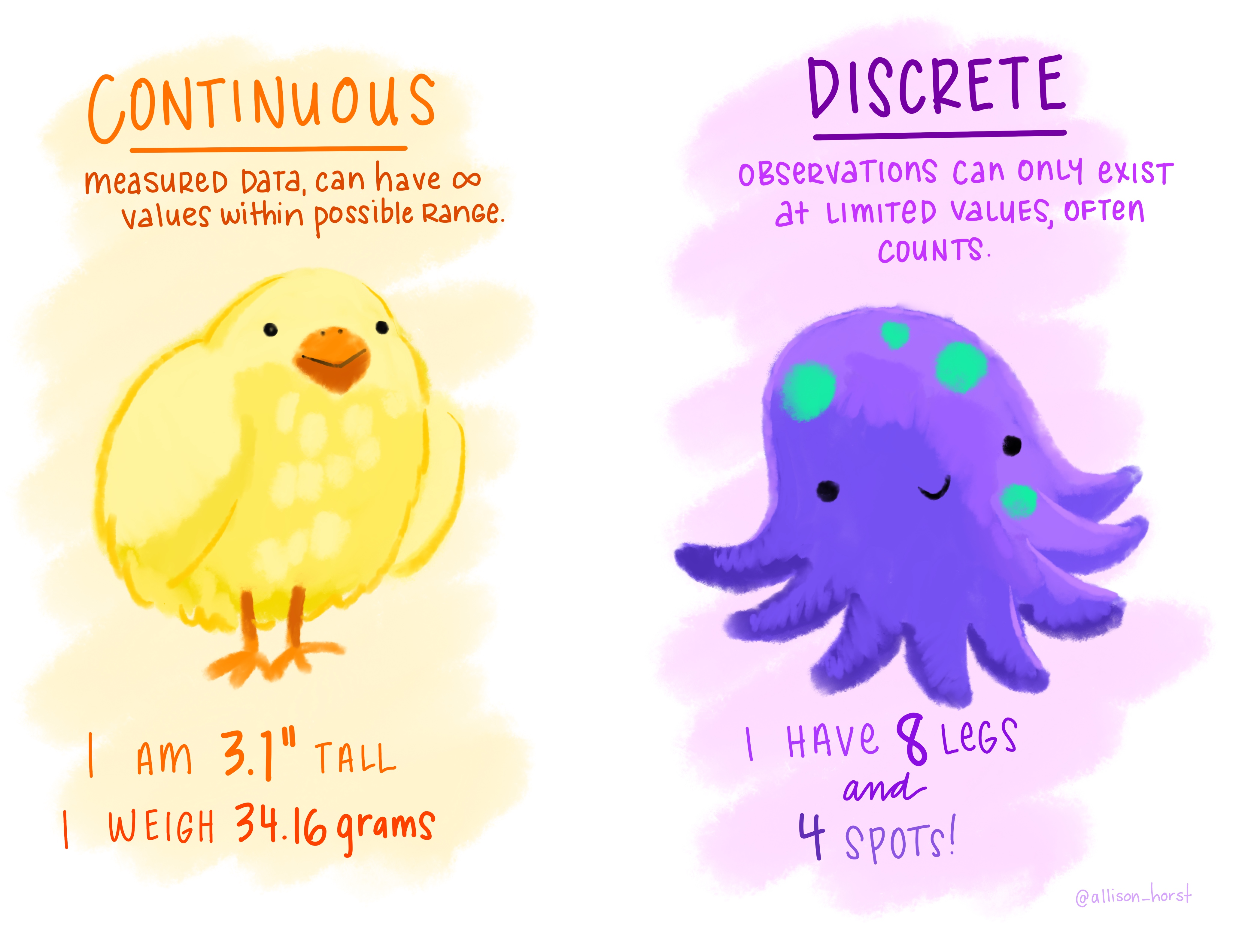
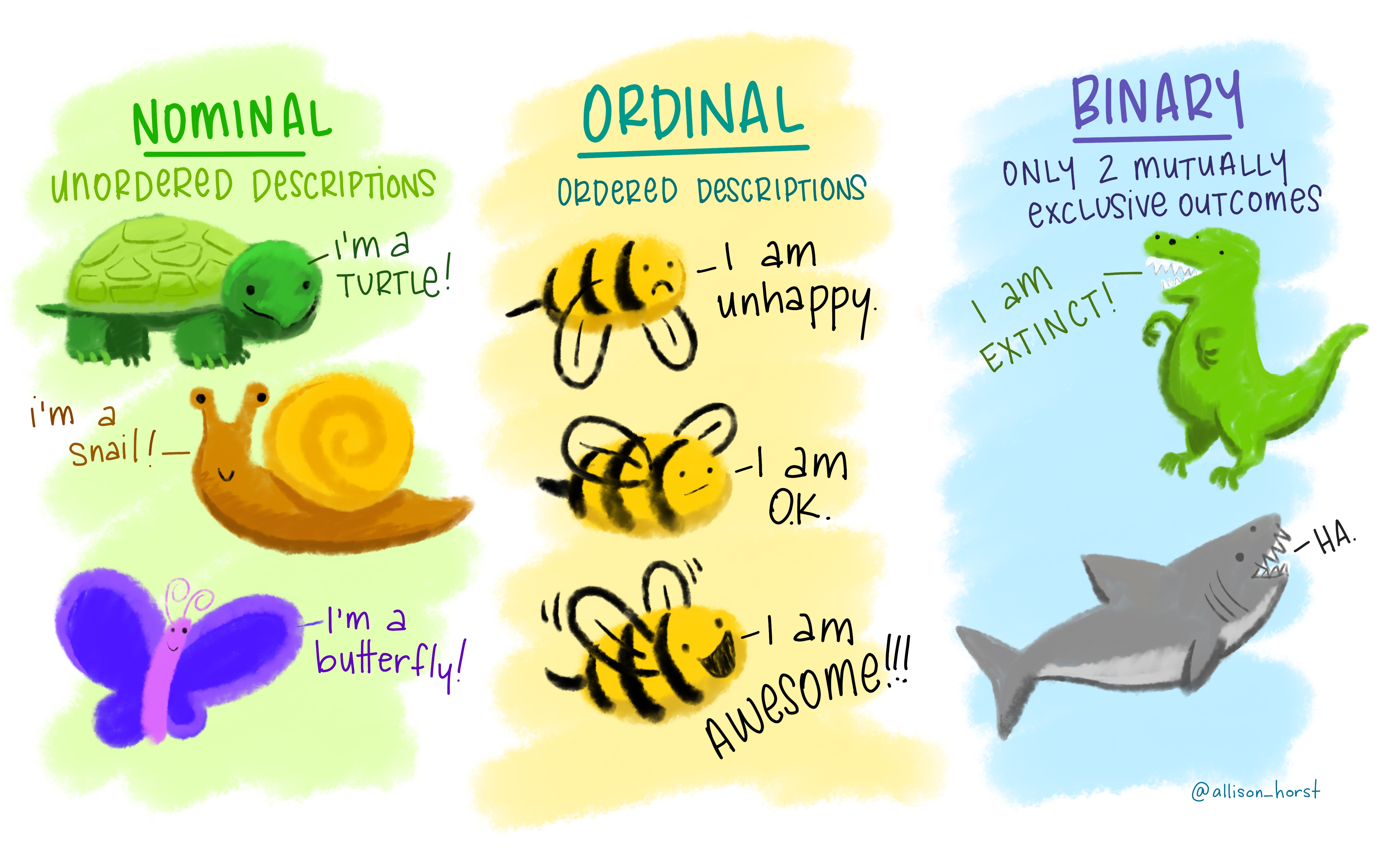
Data Tip: Variable Types

In data we often have variables (i.e. columns in a table) of different types. An important step when starting your analysis is to recognise which kind each variable is.

Numerical	Categorical

Key Points

• Assign values to objects using <-

• Functions perform operations on objects: they take inputs (arguments) and return outputs (values).

• The basic data structure in R is called a vector, which you construct with the c() function.

• The main types of vector values are: numeric (or double), integer, character and logical.

• To subset vectors use []

• When doing vector operations R will ‘recycle’ shorter vectors if it needs to.

• Missing data is supported by functions and is represented by the special value NA

• Vectors can only contain one type of value. If there are mixed types of values in a vector, R will coerce those values into a single type according to the following hierarchy: character > numeric > logical