Manipulating observations (rows) with `dplyr`

Overview

Teaching: 40 min
Exercises: 25 min

Questions

How to order rows in a table?

How to retain only unique rows (no duplicates)?

How to identify observations of a dataset that fulfill certain conditions?

Objectives

Apply the functions arrange() distinct() and filter() to operate on rows.

Understand how logical comparisons are made and the logical data type.

Remember and distinguish between different types of logical operators.

Use conditional operations to obtain specific observations from data using the filter() function.

Combine the filter() and is.na() functions to remove missing values.

Use the ifelse() function to highlight specific observations.

In this lesson we’re going to learn how to use the dplyr package to manipulate rows of our data.

As usual when starting an analysis on a new script, let’s start by loading the packages and reading the data. We will continue with gapminder data from 1960 to 2010:

library(tidyverse)

# Read the data, specifying how missing values are encoded
gapminder1960to2010 <- read_csv("data/raw/gapminder1960to2010_socioeconomic.csv", 
                                na = "")

Ordering Rows

Or order the rows of a table based on certain variables, we can use the arrange() function:

gapminder1960to2010 %>% 
  select(country, world_region, year) %>% 
  # order by year
  arrange(year)

# A tibble: 9,843 x 3
   country              world_region              year
   <chr>                <chr>                    <dbl>
Afghanistan          south_asia                1960
Angola               sub_saharan_africa        1960
Albania              europe_central_asia       1960
Andorra              europe_central_asia       1960
United Arab Emirates middle_east_north_africa  1960
Argentina            america                   1960
Armenia              europe_central_asia       1960
Antigua and Barbuda  america                   1960
Australia            east_asia_pacific         1960
Austria              europe_central_asia       1960
# … with 9,833 more rows

In this case, the rows are sorted by increasing numeric order of the variable year.

When ordering by a character variable, the order will be determined alphabetically:

gapminder1960to2010 %>% 
  select(country, world_region, year) %>% 
  # order by world_region
  arrange(world_region)

# A tibble: 9,843 x 3
   country   world_region  year
   <chr>     <chr>        <dbl>
Argentina america       1960
Argentina america       1961
Argentina america       1962
Argentina america       1963
Argentina america       1964
Argentina america       1965
Argentina america       1966
Argentina america       1967
Argentina america       1968
Argentina america       1969
# … with 9,833 more rows

To arrange based on descending order, you can wrap the variable in the desc() function:

gapminder1960to2010 %>% 
  select(country, world_region, year) %>% 
  # order by year
  arrange(desc(year))

# A tibble: 9,843 x 3
   country              world_region              year
   <chr>                <chr>                    <dbl>
Afghanistan          south_asia                2010
Angola               sub_saharan_africa        2010
Albania              europe_central_asia       2010
Andorra              europe_central_asia       2010
United Arab Emirates middle_east_north_africa  2010
Argentina            america                   2010
Armenia              europe_central_asia       2010
Antigua and Barbuda  america                   2010
Australia            east_asia_pacific         2010
Austria              europe_central_asia       2010
# … with 9,833 more rows

Finally, you can include several variables within arrange(), which will sort the table by each of them. For example:

gapminder1960to2010 %>% 
  select(country, world_region, year) %>% 
  # order by year, then by world region (z-a), then country (z-a)
  arrange(year, desc(world_region), desc(country))

# A tibble: 9,843 x 3
   country      world_region        year
   <chr>        <chr>              <dbl>
Zimbabwe     sub_saharan_africa  1960
Zambia       sub_saharan_africa  1960
Uganda       sub_saharan_africa  1960
Togo         sub_saharan_africa  1960
Tanzania     sub_saharan_africa  1960
Sudan        sub_saharan_africa  1960
South Sudan  sub_saharan_africa  1960
South Africa sub_saharan_africa  1960
Somalia      sub_saharan_africa  1960
Sierra Leone sub_saharan_africa  1960
# … with 9,833 more rows

Retain Unique Rows

Sometimes it is useful to retain rows with unique combinations of some of our variables (i.e. remove any duplicated rows). This can be done with the distinct() function.

# get unique combination of main religion and world region
gapminder1960to2010 %>% 
  distinct(main_religion, world_region)

# A tibble: 27 x 2
   world_region             main_religion
   <chr>                    <chr>        
south_asia               muslim       
south_asia               Muslim       
sub_saharan_africa       christian    
sub_saharan_africa       Christian    
europe_central_asia      muslim       
europe_central_asia      Muslim       
europe_central_asia      christian    
europe_central_asia      Christian    
middle_east_north_africa muslim       
middle_east_north_africa Muslim       
# … with 17 more rows

Choosing Rows Based on Conditions

To choose rows based on specific criteria, we can use filter(). For example, to get all the rows of data from the 2000’s:

gapminder1960to2010 %>% 
  select(country, year) %>% 
  filter(year > 2000)

# A tibble: 1,930 x 2
   country      year
   <chr>       <dbl>
Afghanistan  2001
Afghanistan  2002
Afghanistan  2003
Afghanistan  2004
Afghanistan  2005
Afghanistan  2006
Afghanistan  2007
Afghanistan  2008
Afghanistan  2009
Afghanistan  2010
# … with 1,920 more rows

Conditional Operations

It is important to understand that when we set a condition like above, the output is a logical vector. Let’s see an example using a small vector.

some_years <- c(1985, 1990, 1999, 1995, 2010, 2000)
some_years < 2000

[1]  TRUE  TRUE  TRUE  TRUE FALSE FALSE

So what the filter() function does is evaluate the condition and return the rows for which that condition is true.

It is possible to combine several conditions by using the logical operators & (AND) and | (OR). For example, if we wanted the years between 1990 and 2000:

# both conditions have to be true
some_years > 1990 & some_years < 2000

[1] FALSE FALSE  TRUE  TRUE FALSE FALSE

And if we wanted the years below 1990 or above 2000, then:

# only one or the other of the conditions has to be true
some_years < 1990 | some_years > 2000

[1]  TRUE FALSE FALSE FALSE  TRUE FALSE

Conditional operators

To set filtering conditions, use the following relational operators:

> is greater than

>= is greater than or equal to

< is less than

<= is less than or equal to

== is equal to

!= is different from

%in% is contained in

To combine conditions, use the following logical operators:

& AND

| OR

Some functions return logical results and can be used in filtering operations:

is.na(x) returns TRUE if a value in x is missing

The ! can be used to negate a logical condition:

!is.na(x) returns TRUE if a value in x is NOT missing

!(x %in% y) returns TRUE if a value in x is NOT present in y

Let’s see an example on how we can combine the filter() function with plotting.

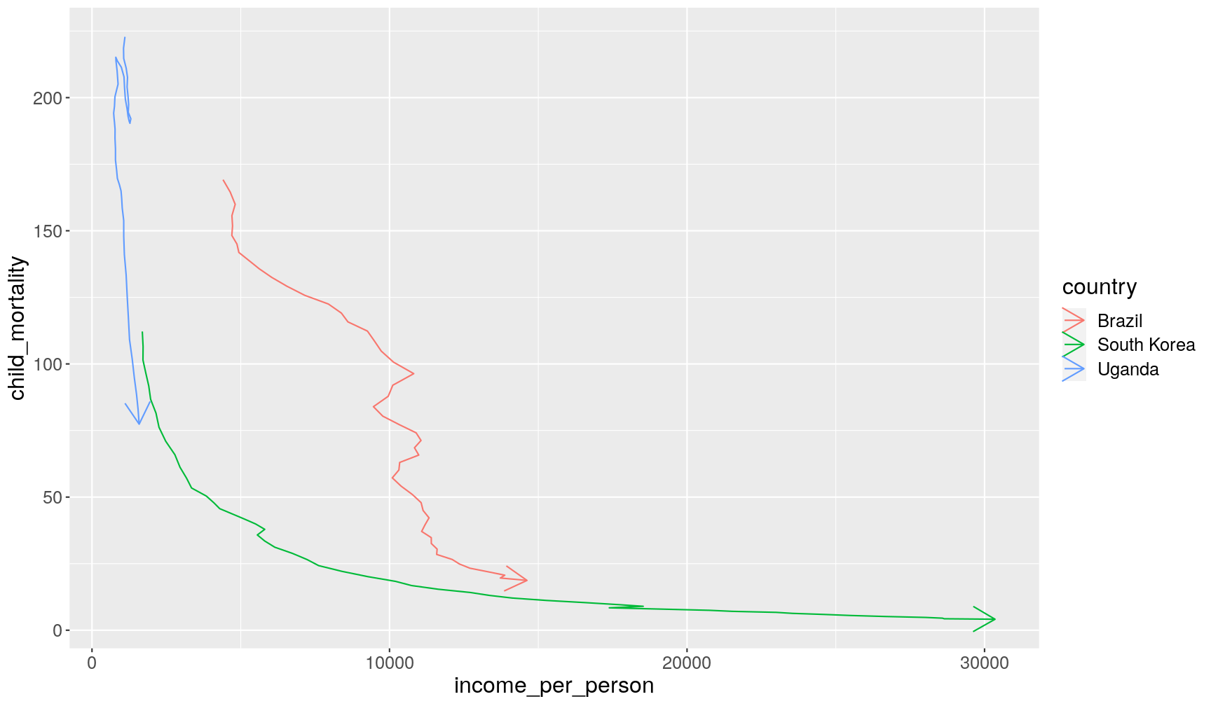
In Hans Rosling’s TED Talk, they compared the change in income_per_person and child_mortality between three countries: Uganda, Brazil and South Korea. We can filter our dataset to retain only these countries by using the %in% operator.

gapminder1960to2010 %>% 
  filter(country %in% c("Uganda", "Brazil", "South Korea"))

We will pipe this filter to ggplot and use geom_path() to look at the change of these countries over time. This geometry is similar to geom_line(), but it connects points in the order they appear on the table (which we can sort beforehand with arrange()), whereas geom_line() connects the points based on the order they appear along the x and y axis. (Try changing the code below to see the difference)

gapminder1960to2010 %>% 
  filter(country %in% c("Uganda", "Brazil", "South Korea")) %>% 
  # ensure data is in order of country and year for geom_path
  arrange(country, year) %>% 
  ggplot(aes(income_per_person, child_mortality)) +
  geom_path(aes(colour = country), arrow = arrow())

plot of chunk unnamed-chunk-14

Exercise

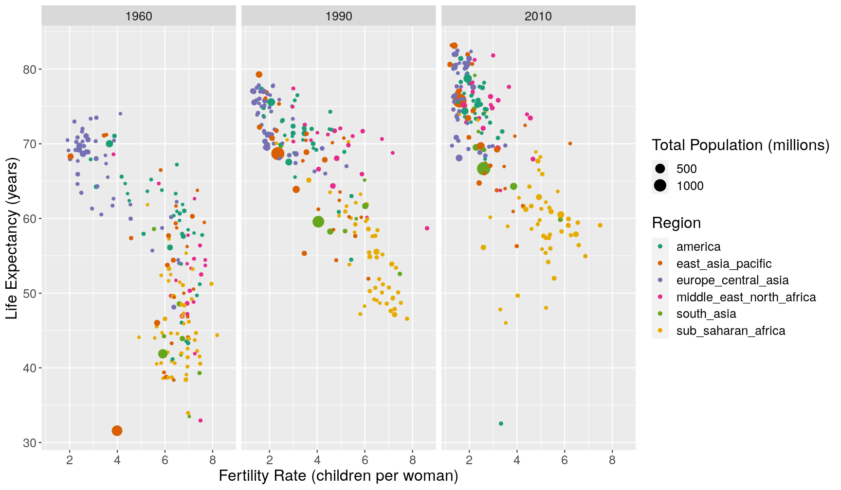
Fix the following code (where the word “FIXME” appears), to produce the plot shown below.

gapminder1960to2010 %>% 
  mutate(population_millions = FIXME) %>% 
  filter(FIXME) %>% 
  ggplot(aes(children_per_woman, life_expectancy)) +
  geom_point(aes(size = population_millions, colour = world_region)) +
  facet_grid(cols = FIXME) +
  scale_colour_brewer(palette = "Dark2") +
  labs(x = "Fertility Rate (children per woman)", y = "Life Expectancy (years)", 
       size = "Total Population (millions)", colour = "Region")

plot of chunk unnamed-chunk-16

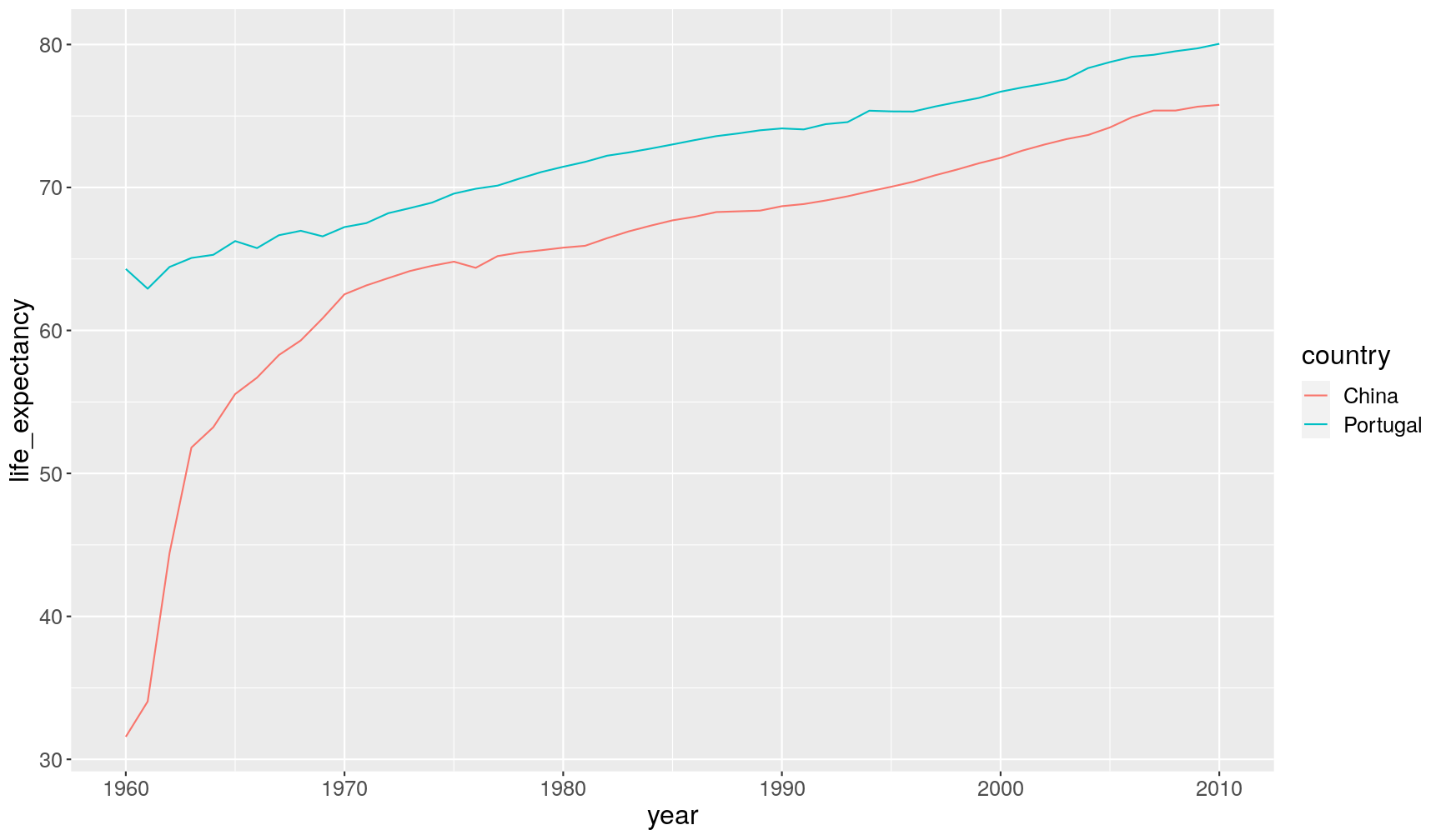
One of the countries seems to stand out from the general trend in 1960. Using some conditions inside filter(), can you find what country it is?
Make a line plot showing how the life_expectancy of that country changed over time compared to another country of your choice.

Answer

A1. Here is the fixed code:

gapminder1960to2010 %>% 
  mutate(population_millions = population/1e6) %>% 
  filter(year %in% c(1960, 1990, 2010)) %>% 
  ggplot(aes(children_per_woman, life_expectancy)) +
  geom_point(aes(size = population_millions, colour = world_region)) +
  facet_grid(cols = vars(year)) +
  scale_colour_brewer(palette = "Dark2") +
  labs(x = "Fertility Rate (children per woman)", y = "Life Expectancy (years)", 
       size = "Total Population (millions)", colour = "Region")

A2. Based on the x and y values in the graph, we can set a condition with filter(), for example:

gapminder1960to2010 %>% 
  filter(year == 1960 & children_per_woman < 5 & life_expectancy < 35) %>% 
  select(country, year, children_per_woman, life_expectancy)

# A tibble: 1 x 4
  country  year children_per_woman life_expectancy
  <chr>   <dbl>              <dbl>           <dbl>
1 China    1960               3.99            31.6

A3. Here is a comparison between China and another country:

gapminder1960to2010 %>% 
  filter(country %in% c("China", "Portugal")) %>% 
  ggplot(aes(x = year, y = life_expectancy)) +
  geom_line(aes(colour = country))

plot of chunk unnamed-chunk-19

Filtering Missing Values

As noted in the callout box above, the is.na() function can be used to ask the question of whether a value is missing or not (!is.na()).

For example, the following would return the rows where main_religion is not missing.

gapminder1960to2010 %>% 
  filter(!is.na(main_religion))

Exercise

How many observations contain values for both life_expectancy and children_per_woman?

Answer

gapminder1960to2010 %>% 
  filter(!is.na(life_expectancy) & !is.na(children_per_woman)) %>% 
  # (optional) pipe the output to nrow() to get the number of rows directly
  nrow()

[1] 9384

Using conditionals with `ifelse`

Conditions are not just useful for filtering rows, but also to modify variables or highlight certain observations in the data.

For example, take the following graph showing the change in income per person:

gapminder1960to2010 %>% 
  ggplot(aes(x = year, y = income_per_person)) +
  geom_line(aes(group = country))

plot of chunk unnamed-chunk-23

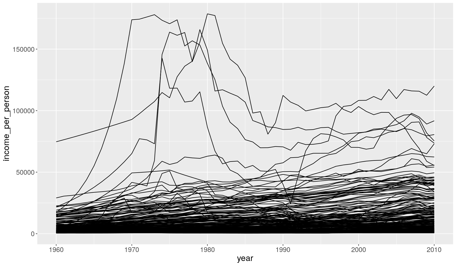
We can highlight one of the countries by creating a new column (mutate()) that stores the result of a condition:

gapminder1960to2010 %>% 
  # the "is_qatar" column will contain TRUE/FALSE values
  mutate(is_qatar = country == "Qatar") %>% 
  ggplot(aes(x = year, y = income_per_person)) +
  geom_line(aes(group = country, colour = is_qatar))

plot of chunk unnamed-chunk-24

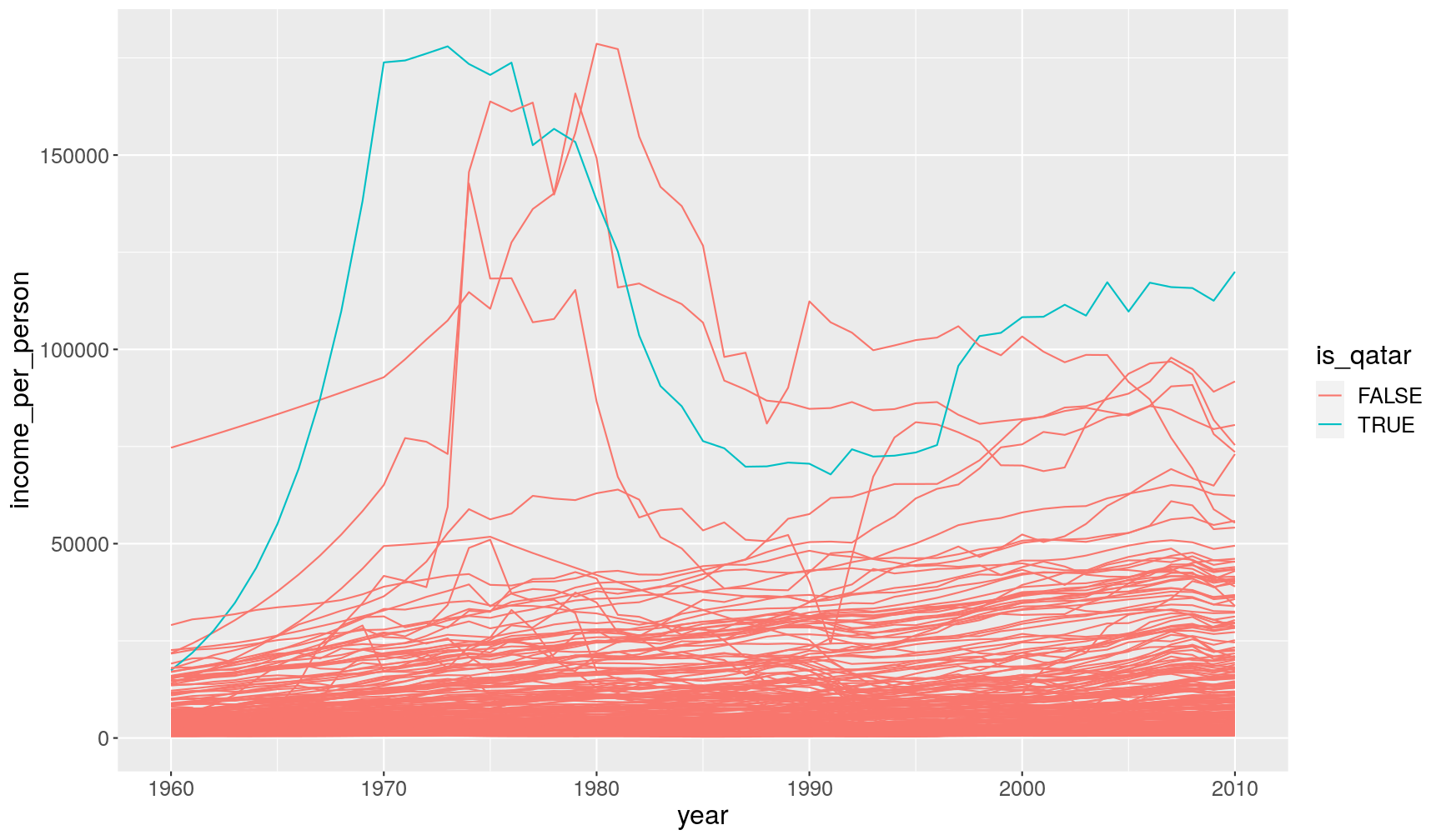
In this case, we used the logical output of that condition as the variable to colour our lines with.

However, sometimes we want more flexibility in defining outcomes from a condition, which is where the ifelse() is handy. This function takes 3 arguments: the condition we want to test, the values it should take if it’s TRUE, and the values it should take if it’s FALSE.

For example, let’s highlight two countries in the graph and label all the remaining countries as “Others” by using ifelse():

gapminder1960to2010 %>% 
  mutate(income_total = population*income_per_person,
         country_highlight = ifelse(country %in% c("China", "United States"), country, "Others")) %>% 
  ggplot(aes(year, income_total)) +
  geom_line(aes(group = country, colour = country_highlight))

plot of chunk unnamed-chunk-25

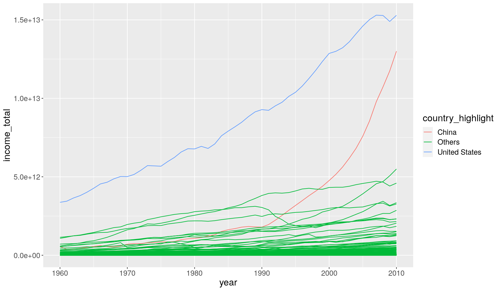
This is what ifelse() did for us: if the value of country is either “China” or “United States” then return their respective value, otherwise return the string “Others”.

ifelse() works in a vectorised manner, meaning that it evaluates the condition at each value and returns the respective result we ask for.

Exercise

Earlier we saw that life_expectancy_male has some values encoded as “-999”:
summary(gapminder1960to2010$life_expectancy_male)
   Min. 1st Qu.  Median    Mean 3rd Qu.    Max. 
-999.00   50.03   61.73   10.64   68.15   80.08 
Try to fix this issue by using ifelse() inside a mutate(), replacing the values of life_expectancy_male with NA if they are equal to “-999” and keeping the original value otherwise.

Save the result by updating gapminder1960to2010 and check that the issue is solved by using the summary() function like above.
Answer
# create new data.frame with missing values for life_expectancy_male
gapminder1960to2010 <- gapminder1960to2010 %>% 
  mutate(life_expectancy_male = ifelse(life_expectancy_male == -999, NA, life_expectancy_male))

# check the result
summary(gapminder1960to2010$life_expectancy_male)
   Min. 1st Qu.  Median    Mean 3rd Qu.    Max.    NA's 
  16.29   51.80   62.56   60.02   68.41   80.08     459 
This is what ifelse() did for us: if the value of life_expectancy_male is equal to -999 then return the value NA, otherwise return the respective value of life_expectancy_male.

Key Points

Order rows in a table using arrange(). Use the desc() function to sort in descending order.

Retain unique rows in a table using distinct().

Choose rows based on conditions using filter().

Conditions can be set using several operators: >, >=, <, <=, ==, !=, %in%.

Conditions can be combined using & and |.

The function is.na() can be used to identify missing values. It can be negated as !is.na() to find non-missing values.

Use the ifelse() function to define two different outcomes of a condition.

previous episode

Introduction to R/tidyverse for Exploratory Data Analysis

next episode

Manipulating observations (rows) with `dplyr`

Overview

Ordering Rows

Retain Unique Rows

Choosing Rows Based on Conditions

Conditional Operations

Conditional operators

Exercise

Answer

Filtering Missing Values

Exercise

Answer

Using conditionals with `ifelse`

Exercise

Answer

Key Points

previous episode

next episode

previous episode

Introduction to R/tidyverse for Exploratory Data Analysis

next episode

Manipulating observations (rows) with `dplyr`

Overview

Ordering Rows

Retain Unique Rows

Choosing Rows Based on Conditions

Conditional Operations

Conditional operators

Exercise

Answer

Filtering Missing Values

Exercise

Answer

Using conditionals with ifelse

Exercise

Answer

Key Points

previous episode

next episode

Using conditionals with `ifelse`