Working with categorical data + Saving data

Overview

Teaching: 30 min
Exercises: 15 min

Questions

• How to fix common typos in character variables?

• How to reorder values in ordinal categorical variables?

• How to save data into a file?

Objectives

• Discuss some common issues with data cleaning and use functions from the stringr package to help solve them.

• Use factors to order categories and encode ordinal data.

• Save data frame into a file.

In this lesson we’re going to learn how to use the dplyr package to manipulate columns of our data.

As usual when starting an analysis on a new script, let’s start by loading the packages and reading the data. In this lesson we’re going to use the full dataset with data from 1960 to 2010:

library(tidyverse)

# Read the data, specifying how missing values are encoded
gapminder1960to2010 <- read_csv("data/raw/gapminder1960to2010_socioeconomic.csv", 
                                na = "")

Manipulating categorical data

The stringr package provides several functions to manipulate strings (i.e. character values). The functions from that package start with the word str_, so they are easy to identify.

For example, let’s have a look at the distinct values of the income_groups variable:

gapminder1960to2010 %>% 
  distinct(income_groups)

# A tibble: 4 x 1
  income_groups      
  <chr>              
1 low_income         
2 lower_middle_income
3 upper_middle_income
4 high_income        

Let’s say we would instead want to have the values “low”, “lower middle”, “upper middle” and “high”. With the help of some str_*() functions we can do this in two steps:

• remove the string “_income”
• replace the underscore “_” with a space “ “

gapminder1960to2010 %>% 
  # remove the word "_income" from the income_groups values; and then...
  mutate(income_groups = str_remove(income_groups, "_income")) %>% 
  # replace the "_" with a hyphen
  mutate(income_groups = str_replace(income_groups, "_", " ")) %>% 
  # check the distinct values for income_groups
  distinct(income_groups)

# A tibble: 4 x 1
  income_groups
  <chr>        
1 low          
2 lower middle 
3 upper middle 
4 high         

Exercise

Create a new table called gapminder_clean, which fulfils the following requirements:

• Fix any typos in the main_religion values. All values should be in Title Case. (hint: str_squish() and str_to_title())
• The world_region column contains values with a space between words (not “_”) and in Title Case. (hint: str_to_title() and str_replace_all())
• The income_groups column contains the categories: “Low”, “Lower Middle”, “Upper Middle”, “High”. (hint: str_remove(), str_to_title() and str_replace_all())

If you haven’t done so already, also make sure that life_expectancy_female is numeric (as.numeric()) and that life_expectancy_male has values “-999” encoded as NA (ifelse()).

The final table should contain 9843 observations (rows) and 13 variables (columns), 4 of them character, 1 logical and the rest numeric.

Answer

gapminder_clean <- gapminder1960to2010 %>% 
  # fix typos in main_religion and world region
  mutate(main_religion = str_to_title(str_squish(main_religion)),
         world_region = str_to_title(str_replace_all(world_region, "_", " "))) %>% 
  # fit typos in income groups, which needs more steps
  mutate(income_groups = str_remove(income_groups, "_income")) %>% 
  mutate(income_groups = str_to_title(str_replace_all(income_groups, "_", " "))) %>% 
  # fix/create numeric variables
  mutate(life_expectancy_female = as.numeric(life_expectancy_female),
         life_expectancy_male = ifelse(life_expectancy_male == -999, NA, life_expectancy_male))

Finally, check that the final table contains the right number of rows, columns and variable types using str():

str(gapminder_clean)

tibble [9,843 × 13] (S3: spec_tbl_df/tbl_df/tbl/data.frame)
 $ country               : chr [1:9843] "Afghanistan" "Afghanistan" "Afghanistan" "Afghanistan" ...
 $ world_region          : chr [1:9843] "South Asia" "South Asia" "South Asia" "South Asia" ...
 $ year                  : num [1:9843] 1960 1961 1962 1963 1964 ...
 $ children_per_woman    : num [1:9843] 7.45 7.45 7.45 7.45 7.45 7.45 7.45 7.45 7.45 7.45 ...
 $ life_expectancy       : num [1:9843] 39.3 40 40.8 41.5 42.2 ...
 $ income_per_person     : num [1:9843] 2744 2702 2683 2665 2649 ...
 $ is_oecd               : logi [1:9843] FALSE FALSE FALSE FALSE FALSE FALSE ...
 $ income_groups         : chr [1:9843] "Low" "Low" "Low" "Low" ...
 $ population            : num [1:9843] 8996967 9169406 9351442 9543200 9744772 ...
 $ main_religion         : chr [1:9843] "Muslim" "Muslim" "Muslim" "Muslim" ...
 $ child_mortality       : num [1:9843] 357 351 345 340 335 ...
 $ life_expectancy_female: num [1:9843] 33.3 33.8 34.4 34.9 35.4 ...
 $ life_expectancy_male  : num [1:9843] 31.7 32.2 32.7 33.2 33.7 ...
 - attr(*, "spec")=
  .. cols(
  ..   country = col_character(),
  ..   world_region = col_character(),
  ..   year = col_double(),
  ..   children_per_woman = col_double(),
  ..   life_expectancy = col_double(),
  ..   income_per_person = col_double(),
  ..   is_oecd = col_logical(),
  ..   income_groups = col_character(),
  ..   population = col_double(),
  ..   main_religion = col_character(),
  ..   child_mortality = col_double(),
  ..   life_expectancy_female = col_character(),
  ..   life_expectancy_male = col_double()
  .. )

Using factors to encode ordinal categorical data

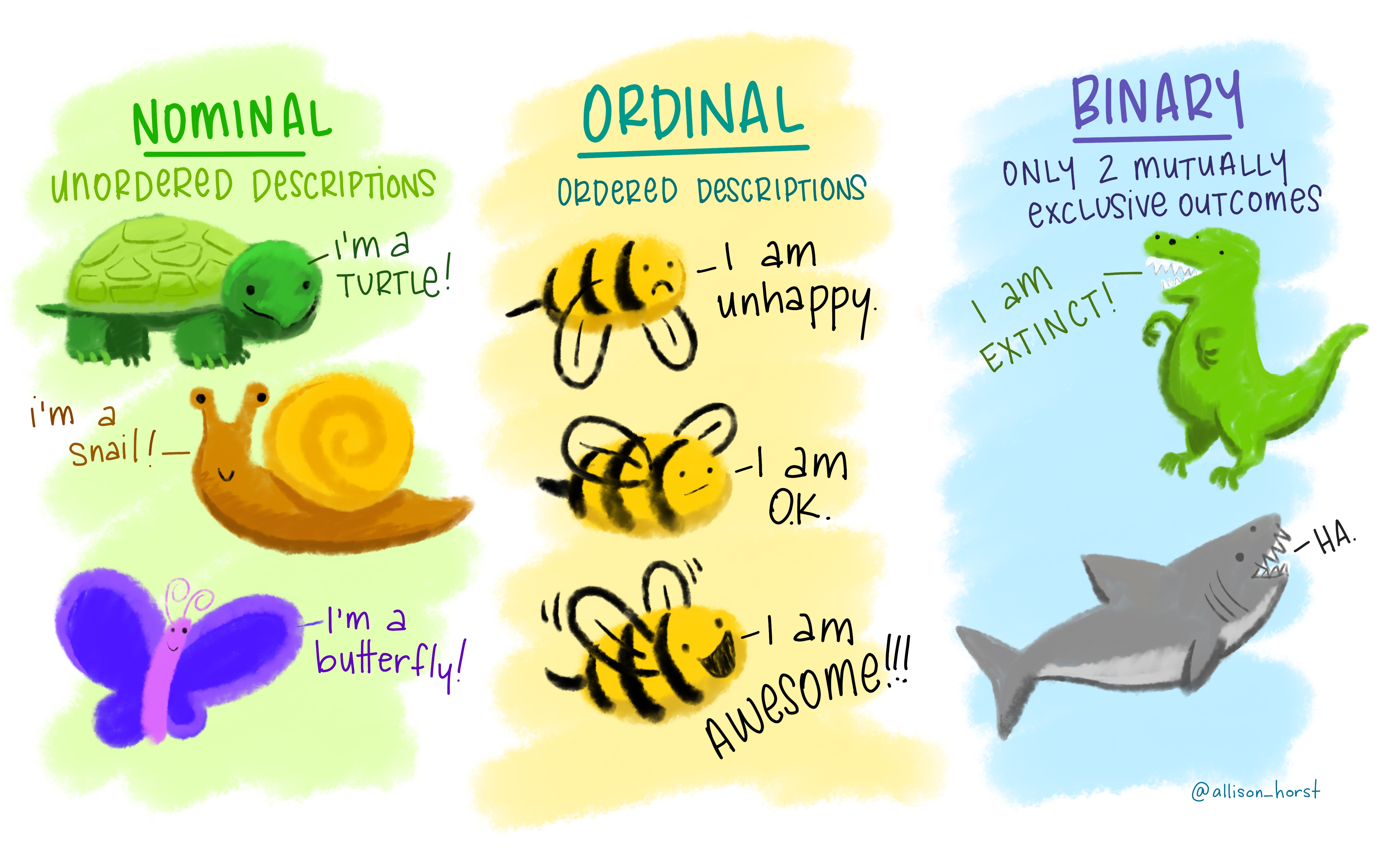
As we discussed in a previous episode, categorical data come in three flavours: nominal, ordinal and binary.

While character vectors can be used to encode non-ordered (nominal) categories, they are not suitable to encode ordered ones. For this, we need to use factors, which are a special type of vector that stores categorical data.

Here is an example using a character vector:

mood <- c("unhappy", "awesome", "ok", "awesome", "unhappy")

# convert mood character vector to a factor
factor(mood)

[1] unhappy awesome ok      awesome unhappy
Levels: awesome ok unhappy

Once created, factors can only contain a pre-defined set of values, known as levels, which correspond to the unique values in the data. By default, R always sorts levels in alphabetical order, like in the example above.

Sometimes, the order of the levels does not matter, other times you might want to specify the order because it is meaningful (e.g., “low”, “medium”, “high”), it improves your visualization, or it is required by a particular type of analysis.

Here is how we would reorder the levels of the mood vector:

factor(mood, levels = c("unhappy", "ok", "awesome"))

[1] unhappy awesome ok      awesome unhappy
Levels: unhappy ok awesome

The forcats package (part of tidyverse) provides several other functions to manipulate factors. These functions all start with fct_, so they are easy to identify. Look at the package documentation to learn more about it.

Exercise

Take the following boxplot showing the distribution of income, per income groups:

gapminder_clean %>% 
  ggplot(aes(income_groups, income_per_person)) +
  geom_boxplot() +
  scale_y_continuous(trans = "log10")

The ordering of the categories on the x-axis is alphabetical. In this case, it would make sense to change this order, to reflect it’s ranking.

Use the factor() function within mutate() to modify the income_groups variable to have a more logical order.

Answer

We can do this by mutating the variable into a factor, where we specify the levels manually:

gapminder_clean %>% 
  # convert income groups to a factor
  mutate(income_groups = factor(income_groups, 
                                levels = c("Low", 
                                           "Lower Middle", 
                                           "Upper Middle",
                                           "High"))) %>% 
  # make the graph
  ggplot(aes(income_groups, income_per_person)) +
  geom_boxplot() +
  scale_y_continuous(trans = "log10")

Saving data

Now that we have a clean version of our table, it’s a good idea to save it for future use. You can use the write_*() family of functions to save data in a variety of formats.

Let’s use write_csv() as an example. The write_csv() function needs the name of the table you want to save and then path to the file you want to save it in (don’t forget the file extension!):

write_csv(gapminder_clean, "data/processed/gapminder1960to2010_clean.csv")

There are many other functions for saving data, you can check the documentation with ?write_delim.

Data Tip: Cleaning Data

The infamous 80/20 rule in data science suggests that about 80% of the time is spend preparing the data for analysis. While this is not really a scientific rule, it does have some relation to the real life experience of data analysts.

Although it’s a lot of effort, and usually not so much fun, if you make sure to clean and format your data correctly, it will make your downstream analysis much more fluid, fruitful and pleasant.

Key Points

• Use functions from the stringr package to manipulate strings. All these functions start with str_, making them easy to identify.

• Use factors to encode ordinal variables, ensuring the levels are set in a logical order.